Working with National Sample Survey (NSS) data in Stata

In recent years, India’s Ministry of Statistics & Programme Implementation (MOSPI) has been releasing micro-data for some of the large-scale sample surveys conducted by the National Sample Survey Organization (NSSO). This is kind of cool because, in the past, if you wanted to work with NSS unit-level data you had to purchase it. This could be an arduous process and the data was not cheap, especially for “foreign” researchers.

There is a lot of documentation that comes with these data, but not very much practical information for how to use it. After I noticed that others were struggling with similar questions, I decided to transform my notes into a blog post that I hope will save others some time.

The examples given here are based on the NSS 68th Round: Employment and Unemployment that was conducted in 2011-2012. For convenience, I am just going to refer to it as the “Employment and Unemployment Survey” or “EUS”.

After 2011-2012 the EUS was replaced by the Periodic Labor Force Survey (PLFS). It is too bad that the NSS abandoned the EUS, because there were some interesting questions there about land ownership and union membership that the PLFS does not include. Nevertheless, the EUS remains a useful resource for historical analysis, and since the EUS is similar in design to other NSSO surveys, the concepts and examples provided here should be useful for analyzing a lot of the other unit-level data released by MOSPI.

Accessing the Data

The data that I am going to be working with in this post are located here. You can download the relevant files by clicking on the “GET MICRODATA” tab and filling out the necessary paperwork.

Next, read the instructions on how to access the data in the README_FIRST file. To access the unit-level data and documentation, you will need the Nesstar Explorer installed, which you can find in the software folder. Once you have that installed, you need to find and run the AutorunPro.exe.

From there, navigate to Data set\Data Files folder and click on the folder that you want to download. For this example, we will be using Block_5_1_Usual principal activity particulars of household members and Block_4_Demographic particulars of household members.

Next you need to click on the link that reads “Click here to access/export data files from Nesstar format.” Now you can download and save the file. I find it helpful to rename the file to something shorter, more intuitive and with fewer spaces. For example, I renamed these two files block_5_1_principal_activity and block_4_demographic_particulars.

Sampling Design

Before working with the NSS data, it is good to be familiar with the basic design of the survey. I will review some of the more important elements here. For more detailed information, you can access the survey documentation. The files titled “Introduction Concepts, Definitions and Procedures”, “Instructions to Field Staff” and “Procedures for Obtaining Estimates of Aggregates, Ratios and their RSEs” in the Other Materials folder should tell you everything you want to know about the survey and how it was conducted.

Here are the key features of the sampling design for the 2011-2012 EUS:

PSU: The primary sampling units (PSUs) are census villages in the rural sector and Urban Frame Survey (UFS) blocks in the urban sector. In the NSS documentation, PSUs are referred to as “First Stage Units (FSUs).”

Sampling Frame: For the rural sector, the sampling frame is all of the census villages. For the urban sector, the sampling frame is a list of UFS blocks.

USU: The ultimate sampling units (USU) are households in the rural and urban sectors. In the NSS documentation, the USU is referred to as the “Ultimate Stage Unit.”

Strata: The sample is first stratified by rural and urban areas within each district. Then all towns with a population over one million constitute their own separate stratum. So say you have a district with two towns with more than one million inhabitants. In that case, you would have four strata in the district: one rural; one for each of the towns; and a third for the remaining towns with fewer than one million inhabitants. The data taken from each strata are referred to as “subsamples” in the NSS documentation.

Sub-strata: There are four substrata within each rural and urban stratum. These are created by listing the villages/towns in ascending order of population (for rural areas) or households (for urban areas) and then demarcating the four strata so that each stratum has roughly equal population.

Selection of PSUs: In rural areas, villages are selected by probability proportional to size with replacement, where size is the population of the village as per the census. For urban areas, blocks are selected by simple random sampling without replacement.

Hamlet Groups and Sub-blocks: If the population of the PSU is more than 1,200, it is divided into a smaller number of relatively equal-size hamlet groups or sub-blocks. The number of hamlet groups or sub-blocks increases with the size of the population of the PSU. Once the population has been divided up into hamlet groups or sub-blocks, two of them are selected. The hamlet group or sub-block with the biggest share of the population is always selected. The second is selected by simple random sampling.

Rounds: Most NSS surveys are carried out in multiple rounds (usually four) over an extended period of time (usually one year).

Weights: The NSS data include a number of weights. The file titled “sampling.html” in the “technical information” folder has some information on the weights. From Nesstar Explorer, you can access this file through the “Sampling” icon under “Study Description.”

The weights (mulptilers) are subsample weights and have to be manipulated to get overall population weights. In the data, we see:

• MLT–Sub-sample multiplier
• MLT_SR–Sub-round multiplier
• Multiplier_comb–Combined multiplier

Multiplier_comb is the weight for “generating subsample-wise estimates based on data of all subrounds taken together.” It is calculated by taking MLT and dividing by 100 if NSS = NSC or dividing MLT by 200 otherwise. This is the main weight that you want to work with if you are using the whole database (as opposed to data from a particular subround).

• NSS–the count of sub-sample wise values falling within a stratum
• NSC–sub-sample combined values falling within a stratum

Whenever a sample value is repeated in both the sub-samples (rural and urban), the multiplier value is (MLT/100), whereas if the sample value is present in only one sub-sample, the multipler value is (MLT/200).

Second Stage Strata: There are three strata for the selection of households within each FSU, hamlet group or sub-block.

• Rural sector
  • SSS1: Relatively affluent households
  • SSS2: Of the remaining households, those with principal income from non-agricultural activity
  • SSS3: Other households
• Urban sector
  • SSS1: HH with MPCE in top 10% of urban population
  • SSS2: HH with MPCE in middle 60% of urban population
  • SSS3: HH with MPCE in bottom 30% of urban population

Selection of Households: For FSUs without hamlet groups or sub-blocks, the distribution of households among the second stage strata is as follows:

• SSS1: 2 households if there are no hamlet groups/sub-blocks; 1 otherwise
• SSS2: 4 households if there are no hamlet groups/sub-blocks; 2 otherwise
• SSS3: 2 households if there are no hamlet groups/sub-blocks; 1 otherwise

Organizing the Data

The NSS data are released in separate “blocks.” Oftentimes you want to merge the blocks so that you can see how variables stored in one block relate to those stored in another block. For our analysis, we are mostly going to be using data from Block 5 but we will also need to grab data on the respondent’s sex from Block 4.

Let’s go ahead and open block_5_1_principal_activity. The variable names are a little long and unconventional and most of them are not labeled. For clarity’s sake, we can rename, label and keep the variables that will be useful for this exercise.

use block_5_1_principal_activity, clear

ren State state
lab var state "state code"

ren District_code dist_code
lab var dist_code "district code"

ren Sector sector
lab var sector "rural or urban"

ren Stratum stratum
lab var stratum "stratum"

ren Sub_Stratum_No substratum
lab var substratum "substratum"

ren FSU_Serial_No psu
lab var psu "primary survey unit (village/block)"

ren Hamlet_Group_Sub_Block_No hamlet_subblock
lab var hamlet_subblock "hamlet group or sub-block number"

ren Second_Stage_Stratum_No ss_strata_no
lab var ss_strata_no "second stage stratum number"

ren Sample_Hhld_No household
lab var household "represents the nth household within each of the second stage stratum"

ren Person_Serial_No person
lab var person "identifier for individual respondent"

ren Age age
lab var age "age of respondent"

ren Usual_Principal_Activity_Status upas_code
lab var upas_code "Usual principal activity status code"

ren HHID hhid
lab var hhid "household identifier"

ren Multiplier_comb pweight
lab var pweight "probability weight (combined multiplier)"

keep state dist_code sector stratum substratum psu pweight hamlet_subblock ss_strata_no household hhid person age upas_code

file block_5_1_principal_activity.dta not found
r(601);

r(601);

We need to destring the variable upas_code because it has to be an integer in order to use it with Stata’s svy commands as we will do below.

destring upas_code, replace

We also need to generate an identifier for the first stage strata since the dataset does not actually include one.

gen fs_strata = state + sector + stratum + substratum
lab var fs_strata "first stage strata"

Now we need to create a unique identifier for each observation that we can use for merging block 5 with other files in the dataset:

gen id = hhid + person
lab var id "observation identifier"

Let’s reorder the data in a more intuitive way and save all of the changes that we made in a new file:

order id state dist_code sector stratum substratum psu fs_strata hamlet_subblock ss_strata household hhid person pweight age upas_code

save block_5_1_exercise, replace

For this exercise, we are going to need to get the sex of the respondent from Block 4 on “demographic particulars.” Let’s open the Block 4 file and save a new file with just the sex of the respondent and the observation identifier.

use block_4_demographic_particulars, clear

destring Sex, replace
recode Sex (2=1) (1=0), gen(sex)
lab var sex "1 = female; 0 = male"

ren Person_Serial_No person
lab var person "identifier for individual respondent"

ren HHID hhid
lab var hhid "household identifier"

gen id = hhid + person
lab var id "observation identifier"

keep sex id
save block_4_exercise, replace

Now we can merge the block 4 and 5 files and save the resulting file as a new file titled NSS_exercise.

use block_5_1_exercise, clear
merge 1:1 id using block_4_exercise
save NSS_exercise, replace

Svyset the NSS Data

The next step is going to be to svyset the data so that Stata is aware of the key elements of the survey design. Without these, Stata will not produce accurate point estimates or standard errors

If you are not familiar with svyset, Stata has a video that provides a basic introduction. I also highly recommend this UCLA tutorial, which provides a more detailed walkthrough as well as a great introduction to survey design.

The three basic elements of the survey that we want Stata to be aware of are the primary survey unit, the probability weight and the first stage strata. We should also tell Stata how to deal with possible single units in a stratum by setting the singleunit option. After we svyset these elements, we can use svydescribe to view detailed information about the design elements.

use NSS_exercise, clear
svyset psu [pw = pweight], strata(fs_strata) singleunit(centered)

svydescribe

I am omitting the svydescribe output here because it is quite long. But if you run it on your machine, you will notice that the output from svydescribe is very similar but not identical to what is listed in the documentation.

In the svydescribe output, we see 3,143 total (sub)strata, 12,737 PSUs and a total of 456,999 individuals. The overview section of the documentation says that 12,654 PSUs out of an allotted 12,808 were surveyed while the file titled “Estimation Procedure_68.doc” says that 12,784 PSUs were allotted. The overview section also states that 100,957 households and 459,784 individuals were surveyed. All of these figures differ slightly from what we find in the files. And doing a similar exercise for the Block_3_Household characteristics, I find that the number of households surveyed is 101,724.

I am not entirely sure how to reconcile the differences between the documentation and what we see in the files. Perhaps in some cases the NSSO could not survey an allotted PSU due to difficult field conditions. Browsing through the svydescribe output, we see some strata in which the output from svydescribe lists three units where the “Estimation Procedure_68.doc” file lists four allotted PSUs, which seems like evidence in favor of this hypothesis. The discrepancies could also be due to human error in writing up the documentation. Or perhaps some additional cleaning of the data was done after the documentation was written. Maybe others will have some insights that I can incorporate into the post.

Reproduce Some NSS Results

Let’s try to replicate some of the household characteristics estimates from the report entitled “Key Indicators of Employment and Unemployment in India, 2011-12.”

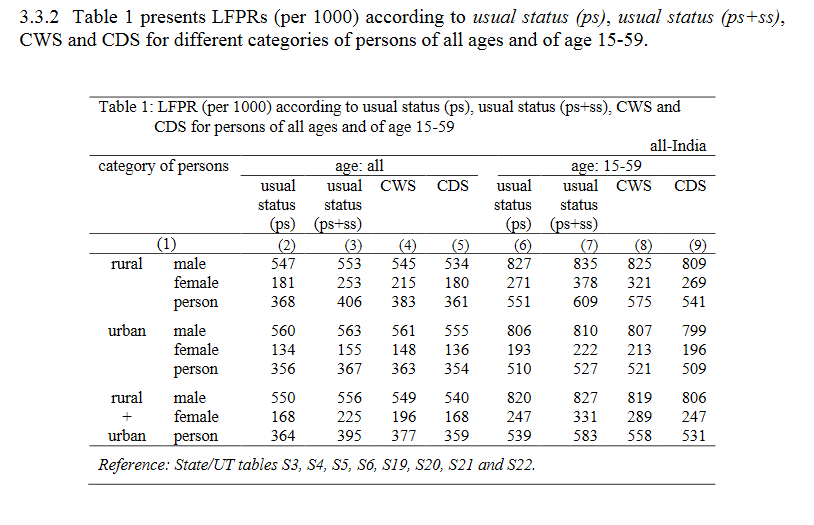
We will focus on Table 1 in section 3.3 on Labor Force Participation and Unemployment.

Next, we will generate indicator variables for “in the labor force” and “unemployed” based on “usual principal activity status”. Here are the relevant codes:

• 11-51: Employed (we won’t use these; but good to know)
• 81: Unemployed
• 91-99: Not in labor force

gen inlf = (upas_code < 90)
lab var inlf "in the labor force"

gen unemployed = (upas_code == 81)
lab var unemployed "unemployed"

We also need an indicator variables for working age, rural and urban:

gen working_age = (age >14 & age <60)
lab var working_age "of working age"

gen rural = (sector == "1")
lab var rural "rural sector"

gen urban = (sector == "2")
lab var urban "urban sector"
save NSS_exercise, replace

Now we can reproduce some of the statistics in the table. Let’s start with the labor force participation rates (LFPR) based on the “usual status” method that we see in the first six rows of column (2).

use NSS_exercise, clear
quietly: collect: svy: mean inlf, over(rural sex) 
quietly: collect: svy: mean inlf, over(rural) 
collect layout (colname) (result[_r_b _r_se _r_ci]) (cmdset) 
collect clear 

file block_5_1_principal_activity.dta not found
r(601);






Collection: default
      Rows: colname
   Columns: result[_r_b _r_se _r_ci]
    Tables: cmdset
   Table 1: 4 x 3
   Table 2: 2 x 3

1
--------------------------------------------------------------------------------------------------------
                                                             | Coefficient Std. error       95% CI      
-------------------------------------------------------------+------------------------------------------
in the labor force @ rural sector=0 # 1 = female; 0 = male=0 |    .5597634    .002912 .5540553  .5654716
in the labor force @ rural sector=0 # 1 = female; 0 = male=1 |    .1340984   .0024558 .1292845  .1389123
in the labor force @ rural sector=1 # 1 = female; 0 = male=0 |    .5465586   .0022148 .5422171  .5509002
in the labor force @ rural sector=1 # 1 = female; 0 = male=1 |     .181117    .002068 .1770633  .1851707
--------------------------------------------------------------------------------------------------------

2
-------------------------------------------------------------------------------
                                    | Coefficient Std. error       95% CI      
------------------------------------+------------------------------------------
in the labor force @ rural sector=0 |    .3555847   .0020774 .3515125  .3596569
in the labor force @ rural sector=1 |    .3678965    .001517 .3649228  .3708702
-------------------------------------------------------------------------------

Notice that here I used the over() subcommand to get the breakdown by sector and sex. I also used the quietly and collect prefixes to enhance the readability of the output. The full output can be obtained by simply deleting these prefixes, e.g. svy: mean inlf.

Although the results are presented in a slightly different order, we find that we are able to accurately reproduce the results from the report. In the urban sector, the LFPR is 56% for males, 13.4% for females and 35.6% for the urban population overall. In the rural sector, the LFPR is 54.7% for males, 18.1% for females and 36.8% for the rural population overall.

In addition to the correct estimate of labor force participation rates, svy also gives us standard errors and confidence intervals for each estimate. This is one of the major advantages of using the svy command as opposed to simply multiplying the survey weights by the variable of interest.

Now let’s use the subpop command to reproduce the labor force participation rates for the working age population that we see in the last three rows of column (6):

use NSS_exercise, clear
quietly: collect: svy, subpop(working_age): mean inlf, over(sex)
quietly: collect: svy, subpop(working_age): mean inlf
collect layout (colname) (result[_r_b _r_se _r_ci]) (cmdset)
collect clear 

file block_5_1_principal_activity.dta not found
r(601);






Collection: default
      Rows: colname
   Columns: result[_r_b _r_se _r_ci]
    Tables: cmdset
   Table 1: 2 x 3
   Table 2: 1 x 3

1
---------------------------------------------------------------------------------------
                                            | Coefficient Std. error       95% CI      
--------------------------------------------+------------------------------------------
in the labor force @ 1 = female; 0 = male=0 |    .8203601   .0020346 .8163717  .8243484
in the labor force @ 1 = female; 0 = male=1 |    .2471564    .002415 .2424225  .2518903
---------------------------------------------------------------------------------------

2
--------------------------------------------------------------
                   | Coefficient Std. error       95% CI      
-------------------+------------------------------------------
in the labor force |      .53865   .0015887 .5355358  .5417643
--------------------------------------------------------------

Finally, let’s scroll down to Table 3 in section 3.5 and reproduce some of the unemployment figures in the report.

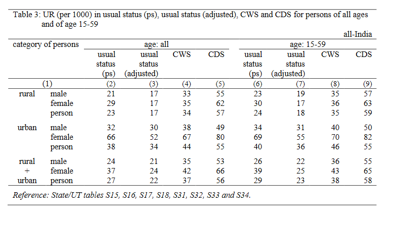
For this one, let’s reproduce the unemployment figures according to the “usual status” method for the working age population for the bottom three rows in column (6):

use NSS_exercise, clear 
quietly: collect: svy, subpop(inlf): mean unemployed, over(working_age sex)
quietly: collect: svy, subpop(inlf): mean unemployed, over(working_age)
collect layout (colname) (result[_r_b _r_se _r_ci]) (cmdset)
collect clear

file block_5_1_principal_activity.dta not found
r(601);






Collection: default
      Rows: colname
   Columns: result[_r_b _r_se _r_ci]
    Tables: cmdset
   Table 1: 4 x 3
   Table 2: 2 x 3

1
--------------------------------------------------------------------------------------------------
                                                       | Coefficient Std. error       95% CI      
-------------------------------------------------------+------------------------------------------
unemployed @ of working age=0 # 1 = female; 0 = male=0 |    .0083967   .0014861 .0054836  .0113099
unemployed @ of working age=0 # 1 = female; 0 = male=1 |    .0169707   .0071731 .0029098  .0310315
unemployed @ of working age=1 # 1 = female; 0 = male=0 |    .0259937   .0009807 .0240713  .0279161
unemployed @ of working age=1 # 1 = female; 0 = male=1 |    .0391951   .0018342 .0355996  .0427905
--------------------------------------------------------------------------------------------------

2
-------------------------------------------------------------------------
                              | Coefficient Std. error       95% CI      
------------------------------+------------------------------------------
unemployed @ of working age=0 |    .0101621   .0019071 .0064237  .0139004
unemployed @ of working age=1 |    .0289707   .0008804  .027245  .0306964
-------------------------------------------------------------------------

Looking at the output where working_age == 1, we see that we are able to reproduce the report’s finding that (based on “usual status” method) the unemployment rate is roughly 2.6% for men, 3.9% for women and 2.9% for the working age population overall. Of course, this is probably not the most convincing method of measuring inequality. But the main point is that we can accurately reproduce the NSSO’s results!

What About the Second Stage Strata?

You might be thinking, “What about the second stage strata? Should we also include those when we svset the data to make our estimates even more precise?”" Let’s try this and see what happens.

First, let’s produce a second stage strata identifier:

use NSS_exercise, clear
gen ss_strata = hamlet_subblock + ss_strata_no
lab var ss_strata "second stage strata"
save NSS_exercise, replace

Now, let’s try using svyset:

svyset psu [pw = pweight], strata(fs_strata) ///
|| household, strata(ss_strata) singleunit(centered)

file block_5_1_principal_activity.dta not found
r(601);


no variables defined
r(111);

r(111);

Stata gives a note that it is not considering the second stage strata. According to this thread, this has to do the with the fact that a finite population correction (FPC) has not been specified in the svyset syntax.

For NSS data, FPC cannot be included for the rural sector because PSUs are indeed selected with replacement as per the survey design. While FPC could theoretically be included for the urban sector, the data needed for calculating the FPC (strata sampling rates or units of population belonging to strata) are not publicly available.

However, there is also an argument to be made that second stage strata may not be all that important for calculations based on NSS data due to the size of India’s population. If the population is so big relative to the sample then you can treat it as infinite, then the second stage strata are immaterial.

Conclusion

In this post, I reviewed the basic survey design for the NSS Employment & Unemployment Survey and then gave a couple of examples of how to reproduce the results from the survey’s main report. Of course, the real fun in being able to access the unit-level NSS data is going to be in producing your own original estimates. Let me know what you come up with!